One of the most common use cases for the Solver SOP is to accumulate values over time.
Accumulating & Substeps
Accumulating a value like color or density over time is pretty straightforward.
- Add to the value from the previous timestep
- Clamp as needed
| |
When you introduce substeps, the accumulation can get a little crazy! Since the solver is doing this addition each timestep, you’ll wind up increasing the value much more quickly than with just one substep. Luckily the solution is pretty straight forward: multiply your accumulation scale by f@TimeInc before adding.
| |
Decaying & Substeps
Accumulating was easy enough right? At first you might think the same could be done for decaying or fading a value over time (like I did…oof!).
If you’re decreasing the value by subtracting, multiplying by f@TimeInc is just fine.
But if you’re doing a fading effect where you’re multiplying by some value between 0 and 1, multiplying by the time increment will actually have the opposite effect!
Imagine you start with a f@density value of 1.0, and you have a decay rate of 0.98. At 1 substep, each frame you are multiplying the previous value by 0.98. So by frame 2, your f@density attribute is 0.98, frame 3 0.9604…and so on.
But if you multiply your decay rate by the time increment, you get a number that’s much much lower!
| |
In this case, each substep we’d be multiplying the value by 0.040768. Even after just a single step we’d probably have all our value eaten away, which is exactly the problem we want to avoid.
Get to the solution already!
Alright alright, we actually have a few ways to solve this one.
Subtract and Clamp
This first way is similar to the additive accumulation method above (subtraction is really just addition in disguise anyways). Instead of decreasing the value by multiplying, we’ll just subtract some small amount each timestep:
| |
Power Function
The second way uses VEX’s pow() function to decay the value over time.
This method will have a different decaying behavior vs just doing a simple multiplication on a single substep. But it tends to look pretty natural so go ahead and try it out
| |
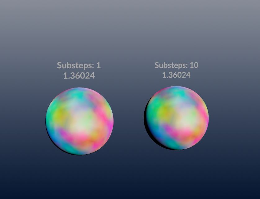
Easy as that! Try it in a Solver SOP with different substep values and see the comparison (or take a look at the attached hipfile). Should be pretty close.
Linear Combination DOP
This method is less for when you’re trying to do this in a SOP solver, and more for if you’re building a setup in DOPs (and want to use this microsolver for something!)
It’s really as simple and changing the dropdown next to the Coefficient parameter from None to e^Timestep. Looks pretty similar to what we just did above!
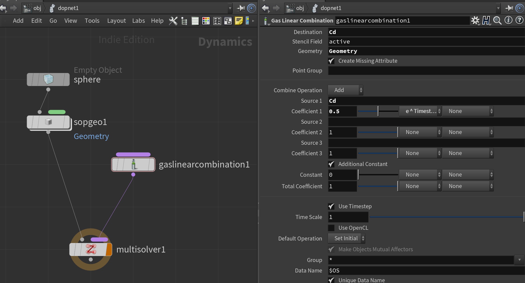
Gas Linear Combination DOP